this is designed for the about link on the homepage to auto expand
Rotational Dynamics
Introduction
Newton formulated some pretty cool and interesting (not to mention absolutely vital to the existence of physics) laws of motion. If you're following the new trend with rotation, you might guess that these laws can be turned into their rotational forms as well. And you'd be right! This unit focuses on Newton's Laws for rotational motion, as well as basic rotational dynamics scenarios.
Newton's Laws in Rotational Form
As you might imagine, these three laws for rotational motion have to do with torque instead of force. The expressions of the three laws are analogous to their normal counterparts.
Newton’s First Law in Rotational form:An object tends to remain in its state of motion unless acted on by a net torque.
Newton’s Second Law in Rotational form:The net torque on an object is equal to its moment of inertia times its angular acceleration.
Newton’s Third Law in Rotational form:For each torque, there is an equal and opposite counter-torque. Sort of...
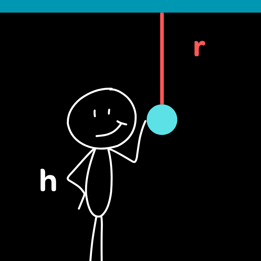
You might be wondering why I was so hesitant there. Well, it's a little bit more complicated when we deal with rotation. Yes, each torque has an equal and opposite "counter-torque" when the entire universe is considered, but we have to recall that for most scenarios we only deal with a few objects. The point of rotation can be different for different objects. Take the case where we hit a pendulum that hangs from the cieling.
Figure 1: Do we have equal and opposite torque pairs? If you push on the ball, the force the ball pushes on you must be the same because of Newton's Third Law. However, the ball will rotate about the pivot in the ceiling a distance $r$ from the point of application, while you will tend to rotate about the contact point with the ground a distance $h$ from the force. This makes the two torques "different", although the reason behind this is that there is the external force of friction and of gravity keeping you from rotating freely. We simply needed to select a larger system to see what was going on.
The other reason why this doesn't look like a "torque pair" is because we considered the torque by the two forces around two different points. This might seem perfectly normal, but in reality we should have considered the torque by the two forces about the same point. In that case, the torques would be equal and opposite. In reality, however, the objects don't rotate about these axes, so in practice this is rarely seen.
So in short: yes, Newton's Third Law applies for rotation, but not in the conventional sense. In most problems, we don't really regard it as that important. It kind of comes up in the later concept of conservation of linear momentum, but we don't typically ask about torque pairs in the way that we ask about force pairs.
The Second Law in Rotational Form
I just spent a while ironing out an idea which won't be important in calculations, but is still important to conceptually understand. Now, I want to go back and talk about the first two laws, which are really very similar to each other. They form the backbone of rotational dynamics problems, giving us an equation as important as $F_{net} = ma$.
The first law is really just a restatement of the second one under equilibrium conditions, much like with forces. Therefore, we will look at the mathematical statememnt of the second law, which we can easily write:
$$ \tau_{net} = I \alpha $$ This equation is as important for rotational dynamics as $F_{net} = ma $$ is for translational dynamics. Essentially, we have the statement that a net torque tends to change the angular velocity of an object. Note that while torque is technically a vector and could cause rotation about several different axes (like a top precessing, or the Earth rotating around the sun while also spinning on its own axis), here we do not consider those complex examples.
In our case, rotation is always going to be in a single plane, like a disk spinning on a flat surface. We can deal with some more complex examples like the Earth, because the rotation of the Earth about its own axis (24 hour period) is so much faster than around the sun (365 day period). Thus, we deal with torqe only in a single plane, meaning we can reduce it to clockwise/counterclockwise. Remember, we usually say counterclockwise is positive whenever direction actually matters.
You horizontally push on a flat metal disk of mass 2.0 kg and radius 3.0 meters that lies flat on a tabletop a perpendicular distance of 0.7 meters from its edge. How hard must you push if the disk is to have an angular acceleration of $\alpha = 0.7 ~\textrm{rad/s}^2$?
The first step is find the actual radius at which the force is being applied. It's a distance of 0.7 meters from the edge, so it would be $2.0 - 0.7 = 1.3 \textrm{m}$ from the center of the disk. We'll call this value $r$ for convenience.
Next, we set up Newton's Second Law in rotational form. We can evaluate the torque symbolically, in terms of the force $F$ needed to cause that angular acceleration.
$$ \tau = I \alpha $$ $$ Fr = \dfrac12 MR^2 \alpha $$ Now, just isolate $F$ and solve for it. At this point, the algebra should be a piece of cake.
We basically have an equivalent form of Newton's Second Law for rotation, which we read off of the statement of the law:
$$ \tau_{net} = I \alpha $$ The first law serves a purpose in introducing a new concept, but we will get to that later on. For now, let's take a look at this law. It essentially just states that a net torque will cause a change in angular velocity for an object. As always, $I$ is measured about the axis of rotation.
This equation takes pretty much the same function as $F_{net} = ma$, only for rotation. (If you look, the form of the equation is identical: every linear quantity is replaced with its rotational counterpart!) However, we only deal with the directions of clockwise and counterclockwise for rotation, so there is no need to do any vector algebra to get the net torque once we know how much torque each force exerts.
With that, let's try a very simple example that'll get us acclimated to this new equation.
You push horizontally on a solid disk's edge, a perpendicular distance $r$ from the center, with some force $F$. The disk has a mass $M$ and radius $R$. Write the angular acceleration of the disk.
First, we know the disk has a moment of inertia of $ I = \frac12 MR^2 $, so we'll keep that in mind. Next, we can easily find the torque that is caused by the force, because the distance $r$ is perpendicular. Thus, we have basically every part we need now.
$$ \tau = I \alpha $$ $$ Fr = \dfrac12 MR^2 \alpha $$ Now, just do some algebraic manipulation of the variables, and we'll be at our final answer!
$$ \alpha = \bbox[3px, border: 0.5px solid white]{\dfrac{2Fr}{MR^2} } $$ Don't be intimidated by the complex-looking final result. We know how we got here, and that's the most important part.
Rotational and Static Equilibrium
The First Law in rotational form actually provides us plenty of insights into a new concept: rotational equilibrium. The condition for this is analogous to that of translational equilibrium. I'll put the two conditions right here:
Translational Equilibrium: $$ \sum F_i = 0 $$ Rotational Equilibrium: $$ \sum \tau_i = 0 $$ These two are not the same! While an object being in translational equilibrium means that it is not accelerating, an object being in rotational equilibrium means that its angular velocity is not changing! These two are pretty similar conditions, but linear and angular quantities are not equivalent. An object can accelerate while maintaining its angular velocity, and vice versa.
This leads to an important conclusion: objects can be in one kind of equilibrium without being in the other. Think of a disk on a CD player. It cannot move around, but its angular velocity can change. The inverse is also true: think of a hockey puck that spins on the ice and is given a sharp tap by a player. If the hit was directly in the middle of the puck, it will accelerate while continuing to rotate at the same angular velocity.
That isn't to say that both cannot be true, however! There is a special name for the kind of equilibrium that arises when both torques and forces sum to zero. We call this special case static equilibrium, and it basically is just when both equations above are satisfied simultaneously.
Rotational and Static Equilibrium
The rotational version of the First Law leads us to conclude that whenever torques sum to zero, the angular velocity doesn't change. That sounds simple enough, but this condition is an equilibrium condition. It can be written mathematically.
$$\tau_{net} = 0 $$ You might also remember another equilibrium condition: there is no acceleration when the net force is zero. This is also an equation:
$$ F_{net} = 0 $$ Now, these look similar, but they are two different things! When torques sum to zero, we have the condition of rotational equilibrium. When forces sum to zero, we have translational equilibrium. Now, torque is not the same as force, so these are two separate conditions. One can be satisfied without the other being satisfied. Need examples?
Think about a CD on a CD player. The disk can rotate and change its angular velocity, but will not have any acceleration (unless you throw the CD player). The other case is true. If you have a hockey puck on ice and hit it at its center, you will cause its velocity to change but it will keep rotating at the same angular velocity.
When both conditions are satisfied, we have a special case called static equilibrium. In this case, objects usually do not accelerate or rotate, though the strict conditions are only that there is no net force or torque.
The most common static equilibrium case is the ladder leaning against a wall. Experience tells us that it will fall over in some cases, but physics can tell us exactly when it would begin to fall over. For the simplest case, we have no friction on the wall and friction between the ladder and the ground. However, before we can tackle a case like this, we need to talk about how to set up rotational dynamics problems.
In translational dynamics, the location where forces were applied did not matter to the problem. This still doesn't matter for the force balance aspect, but it certainly matters for determining torque. Thus, we should now draw force-vector diagrams where forces are drawn at the exact point where they are applied. This also means drawing out the object in question, as well as things around it if they affect the problem. This is what we call a force-vector diagram.
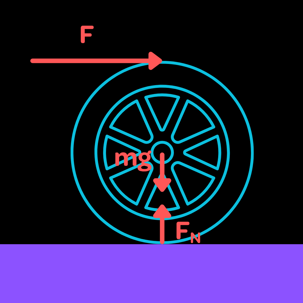
Figure 2: A complete force-vector diagram for a wheel being pushed along a frictionless surface. The diagram above should show you some of the general ideas behind the force-vector diagram. Obviously, the applied force is applied at... well, it's applied where it's applied. Other forces follow some general rules. The gravitational force is always applied at the center of mass, and the normal and frictional forces are applied where there is contact.
The force-vector diagram is really not too different from the free-body diagrams we are used to. We just need to consider the exact positions of the forces in order to calculate torque. It's also helpful to label known lengths and angles on force-vector diagrams, for easy torque calculations. Now, we can work on that ladder problem.
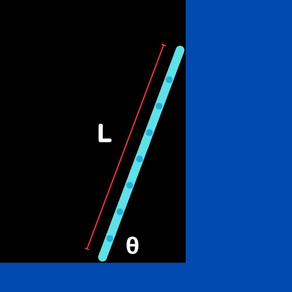
Consider a ladder of mass $m$ and length $L$ that leans against a wall, making an angle $\theta$ with the ground. What must be the required coefficient of static friction between the ladder and floor such that it doesn't slip and fall over?
Figure 3: The elusive (to solve) ladder. First, we want to make a force-vector diagram of the ladder. We know that it has a gravitational force exerted at the center, and normal and frictional forces from the ground. However, that's not all. It's easy to miss the fact that there has to be a normal force from the wall as well, since the ladder leans on it! Thus, we can make our force-vector diagram.
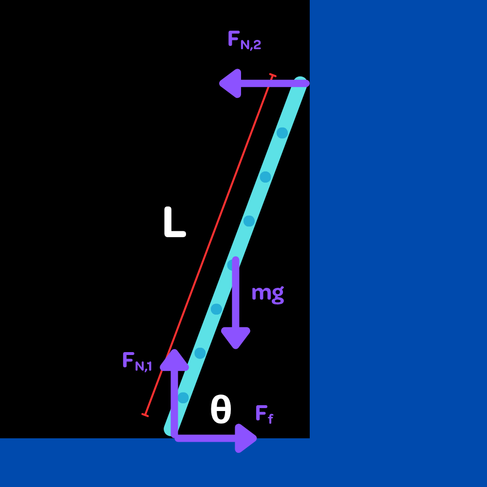
Figure 4: We have now solved the ladder by adding a whole lot of vectors. This lets us do our force and torque analysis. Neither is enough to solve the problem on its own, because this is a static equilibrium case. We have to have both torque and force balance! We'll start with the simpler force equation, using Newton's Second Law. For this, we can ignore where the forces are and treat the entire thing like one big free-body diagram.
In the y-direction, we only have $mg$ and $F_{N,1}$, and in the x-direction we have $F_f$ and $F_{N,2}$.
$$ mg = F_{N,1}$$ $$ F_f = F_{N,2} $$ We can re-write $F_f$ as $ \mu F_{N,1}$ and then simplify the second equation using the first equation.
$$ \mu mg = F_{N,2} $$ Now, we're at a stalemate with forces. We can't find anything else out with this method. However, this is where torque comes to the rescue. In cases of static equilibrium where there is no rotation, we can pick the rotation axis to be wherever we want since torques have to be balanced around any point for there to be no rotation.
We pick the point at the bottom of the ladder, as that allows us to eliminate the two forces located there from our equation. If they're located at the chosen reference point, then they have zero lever arm or distance from the pivot. Then, we have to find the two torques caused by gravity and $F_{N,2}$.
$$ mg \dfrac L2 \cos \theta = F_{N,2} L \sin \theta $$ I haven't gone into depth on how I got these as the torques, but you should be able to get them using the techniques I introduced earlier. This equation allows us to relate $F_{N,2}$ and $mg$, which is exactly what we needed.
$$ F_{N,2} = \dfrac{mg}{2\tan\theta} $$ $$ \mu mg = \dfrac{mg}{2 \tan \theta} $$ We finally arrive at our result:
$$ \bbox[3px, border: 0.5px solid white]{\mu = \dfrac{1}{2 \tan \theta} }$$ Let's think about what this result tells us. We know that $\tan \theta$ increases as the angle increases up to $90 \degree$, which is the maximum angle the ladder can make with the floor. This means that the required friction actually decreases as the ladder gets steeper! This is why we always place our ladders at a pretty steep angle. It's not just to get to higher places, there is a crucial element of safety behind it as well! Create the force-vector diagram for a ladder of mass $m$ and length $L$ that leans against a wall and makes some angle $theta$ with the floor. The ladder has no friction with the wall, but has some friction with the ground. (The ladder stays upright stably.)
Figure 3: The elusive (to solve) ladder. There are a lot of forces involved in this one. We can start with listing the more obvious ones. First, we definitely have a gravitational force equal to $mg$. We have to put this force at the correct location since it's a force-vector diagram, but this isn't too difficult. The gravity always acts at the center of mass, so it goes to the center of the ladder and points straight down.
Next, we have the normal force from the ground, which I'll call $F_{N,1}$. This force is simply located where the ladder touches the ground and points straight upwards. It's a conventional normal force in pretty much all regards.
We also have friction between the ground and ladder, so we have a frictional force $F_f$ at this point as well. The direction of this might not be clear, but it will be later. For now, just keep in mind that it's also at the same point as $F_{N,1}$.
Finally, there is one more force that you might not have thought of. The ladder leans against the wall, so there will be a normal force from the wall! This force is located where the ladder contacts the wall and points directly perpendicular to the wall. In other words, it must point left.
Well, if this force points left and the ladder is stable, that means something has to balance it. This "something" must be the friction, since it's the only other force that points horizontally. Thus, we conclude that the friction has to point to the right. Here's our completed diagram:
Figure 4: We have now solved the ladder by adding a whole lot of vectors. If you want to actually solve this problem for what the required coefficient of friction is, check out our algebra-based level!
Conclusion
These are the basic ideas behind rotational dynamics. If you have a good handle on torque and moment of inertia, this topic should be no issue. It's really a repeat of translational dynamics with a bit more nuance thrown in, so we already developed the techniques to tackle this topic a while ago. That being said, the problems here can get quite complex, so make sure you're clear on the approach you need to take.
The next lesson will continue to talk about rotational dynamics, but instead taking a look at a specific genre of motion within rotational dynamics. Ever seen something roll? Well, now we're going to figure out the physics behind that.